How to open the Power Query editor in Excel
Guide · By Tahir Nas · Examples run in our simulator · Updated
Power Query lives on Excel's Data tab, in the Get & Transform Data group (Microsoft Support: About Power Query in Excel). There are three everyday routes into its editor. They all open the same window, so pick the one that matches what you are doing.
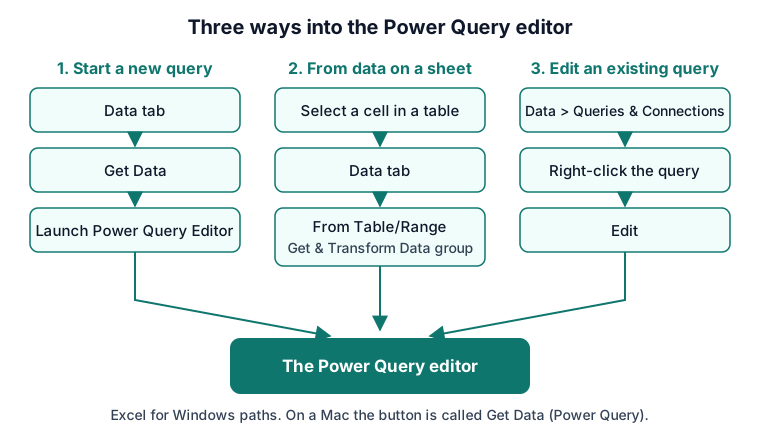
Route 1: Data > Get Data > Launch Power Query Editor
Use this when you want the editor without importing anything yet, for example to write a query from scratch or to look at the queries a workbook already has. Microsoft's steps are Data > Get Data > Launch Power Query Editor (Microsoft Support: Create, load, or edit a query in Excel). The same Get Data menu also has From Other Sources > Blank Query, which opens the editor with an empty query ready for M.
Route 2: From Table/Range
Use this when the data is already on a sheet. Click any cell in an Excel table, then select Data > Get & Transform Data > From Table/Range. Excel opens the Power Query editor with your data in a preview pane, and nothing on the original sheet changes (Microsoft Support: Import from an Excel table). The lesson importing from Excel covers tables, sheets and named ranges in other workbooks.
Route 3: edit a query you already have
To change a saved query, select Data > Queries & Connections, open the Queries tab, right-click the query and select Edit. If a cell of the query's output table is selected, the Query tab on the ribbon has an Edit button too (Microsoft Support: Create, load, or edit a query in Excel).
What each part of the editor is for
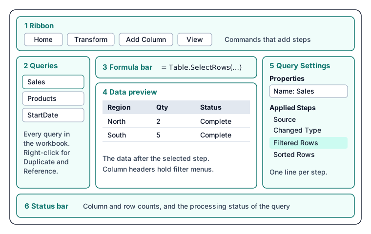
- Ribbon. Tabs of commands such as Home, Transform, Add Column and View. Most buttons add a step to the query.
- Queries pane. Every query in the workbook. Right-click one to duplicate it, reference it or create a function from it.
- Formula bar. The M formula of the selected step. You can type or edit a step's formula here.
- Data preview. The data as it looks after the selected step. Each column header has a menu for sorting and filtering.
- Query Settings. The query's name under Properties, and the Applied Steps list: one line per step, in the order they run.
- Status bar. Column and row counts and the processing status of the query.
Microsoft describes the ribbon, Queries pane, current view, Query Settings and status bar as the editor's main parts (Microsoft Learn: Use Power Query to transform data). Selecting a step in Applied Steps shows the data at that point, which is the fastest way to find where a problem starts (Microsoft Learn: Applied steps).
See the M behind the buttons
Every step you click is written as M. To see the whole query at once, select View > Advanced Editor (Microsoft Learn: Use Power Query to transform data); Microsoft's custom function article also opens it from the Home tab (Microsoft Learn: Using custom functions). A query with the four steps in the diagram above reads like this:
let
    Source = #table(
        {"Order", "Region", "Status", "Qty", "Price"},
        {
            {"A-101", "North", "Complete", "2", "12.50"},
            {"A-102", "South", "Cancelled", "1", "40.00"},
            {"A-103", "North", "Complete", "3", "8.00"},
            {"A-104", "South", "Complete", "4", "5.00"}
        }
    ),
    #"Changed Type" = Table.TransformColumnTypes(Source, {{"Qty", Int64.Type}, {"Price", type number}}, "en-US"),
    #"Filtered Rows" = Table.SelectRows(#"Changed Type", each [Status] = "Complete"),
    #"Sorted Rows" = Table.Sort(#"Filtered Rows", {{"Qty", Order.Descending}})
in
    #"Sorted Rows"
Result
| Order | Region | Status | Qty | Price |
|---|---|---|---|---|
| A-104 | South | Complete | 4 | 5 |
| A-103 | North | Complete | 3 | 8 |
| A-101 | North | Complete | 2 | 12.5 |
Output produced by the Power Query Exercises simulator, an independent implementation of a documented subset of M.
When a pane is missing
If Query Settings has been closed, select View > Query Settings to bring it back (Microsoft Learn: Applied steps). The Queries pane has a collapse icon in its top corner, so a narrow strip on the left usually means it is collapsed rather than gone (Microsoft Learn: Use Power Query to transform data).
Practise with the same layout
The exercises on this site use a browser editor laid out like Excel's: queries on the left, the preview in the middle and applied steps on the right. Start with applied steps are a recipe and read the M behind the steps, then try the tasks below. When you are ready to build a real query in Excel, follow your first Power Query in Excel.
Practise it in the simulator
Each task opens the exact exercise in the browser workspace and is checked against fresh data, not just the example. Free tasks need no account.
- beginner~8 minFree
Reorder steps so cleaning happens before grouping (kite shop)
The query groups regions before cleaning them, so " north" and "North" are counted separately. Fix the step order.
- beginner~5 minFree
Return the last step, not an earlier one (kite shop)
The query builds a Line Total column, but the result doesn't show it: the `in` clause returns an earlier step.
Related pages
Lessons
More resources
Function reference
Sources
Microsoft's official documentation for the features and functions used on this page.
- Use Power Query to transform data (Concept, Microsoft Learn)
- Applied steps (Concept, Microsoft Learn)
- Where to get data (Concept, Microsoft Learn)
- Table.TransformColumnTypes (Function reference, Microsoft Learn)
- Table.SelectRows (Function reference, Microsoft Learn)
- Table.Sort (Function reference, Microsoft Learn)
- About Power Query in Excel (Excel, Microsoft Support)
- Create, load, or edit a query in Excel (Power Query) (Excel, Microsoft Support)
- Import from an Excel table (Excel, Microsoft Support)
- Import and shape data in Excel for Mac (Power Query) (Excel, Microsoft Support)
- Using custom functions (Excel, Microsoft Learn)
Excel menu paths on this page were checked against these pages on 8 November 2026.
Power Query Exercises is an independent educational platform and is not affiliated with, endorsed by, sponsored by, or approved by Microsoft Corporation. All third-party trademarks belong to their respective owners.