Your first Power Query in Excel, from table to refresh
Guide · By Tahir Nas · Examples run in our simulator · Updated
This walkthrough builds one small query end to end: a table of orders becomes a summary of completed sales by region, loaded back into Excel and refreshed after new orders arrive. Every step names the Excel command, and the table at the end maps each step to a lesson and an exercise on this site.
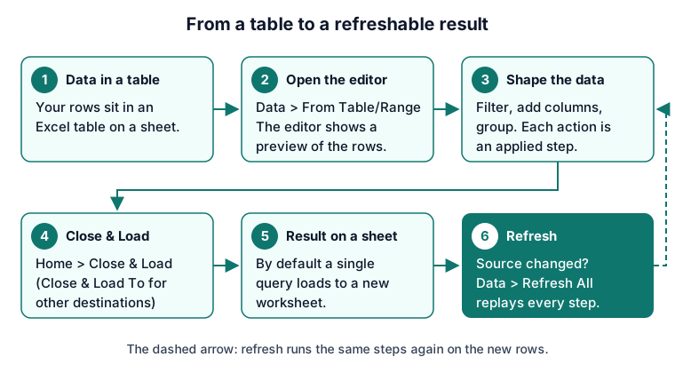
Step 1: start from an Excel table
Put the orders in an Excel table with one header row: Order, Region, Status, Qty and Price. Microsoft's From Table/Range steps start with the cursor in an Excel table (Microsoft Support: Import from an Excel table). If the data is in another workbook or a CSV file instead, use Data > Get Data and pick that source; the lessons on importing from Excel and importing CSV files cover both.
Step 2: Data > From Table/Range
With a cell in the table selected, choose Data > Get & Transform Data > From Table/Range. The Power Query editor opens with the data in a preview pane (Microsoft Support: Import from an Excel table). The first applied step reads the table. A query that reads a table from its own workbook uses Excel.CurrentWorkbook, which only exists inside Excel, so our simulator refuses it rather than pretend:
let
    Source = Excel.CurrentWorkbook(){[Name = "Sales"]}[Content],
    Typed = Table.TransformColumnTypes(Source, {{"Qty", Int64.Type}})
in
    Typed
Not run by the simulator
Excel.CurrentWorkbook is not supported in the Power Query Exercises simulator. See the compatibility page for the supported subset. This code is shown for real hosts only; see the simulator compatibility page.
Output produced by the Power Query Exercises simulator, an independent implementation of a documented subset of M.
Step 3: shape the data
Now add three steps. Each one appears in Applied Steps as you make it (Microsoft Learn: Applied steps):
- Keep completed orders. Open the filter arrow on the Status header and tick only Complete (Microsoft Learn: Filter by values in a column).
- Add a value column. Choose Add Column > Custom Column and enter
[Qty] * [Price](Microsoft Learn: Add a custom column). Then set its type, because the Excel editor's custom column dialog doesn't set one for you. - Total by region. Choose Transform > Group By, group on Region and sum the new column (Microsoft Learn: Grouping or summarizing rows).
Here are the same steps in M, run on the four orders from the table above. In Excel, Source would be the From Table/Range step; here it is written inline so the query runs in the browser:
let
    Source = #table(
        {"Order", "Region", "Status", "Qty", "Price"},
        {
            {"A-101", "North", "Complete", "2", "12.50"},
            {"A-102", "South", "Cancelled", "1", "40.00"},
            {"A-103", "North", "Complete", "3", "8.00"},
            {"A-104", "South", "Complete", "4", "5.00"}
        }
    ),
    Typed = Table.TransformColumnTypes(Source, {{"Qty", Int64.Type}, {"Price", type number}}, "en-US"),
    Completed = Table.SelectRows(Typed, each [Status] = "Complete"),
    WithValue = Table.AddColumn(Completed, "Value", each [Qty] * [Price], type number),
    ByRegion = Table.Group(WithValue, {"Region"}, {{"Sales", each List.Sum([Value]), type number}})
in
    ByRegion
Result
| Region | Sales |
|---|---|
| North | 49 |
| South | 20 |
Output produced by the Power Query Exercises simulator, an independent implementation of a documented subset of M.
Step 4: Home > Close & Load
Select Home > Close & Load to send the result back to Excel (Microsoft Support: Create, load, or edit a query in Excel). Power Query loads the result to a new worksheet by default; to choose another destination, use Close & Load To instead (Microsoft Support: Import from an Excel table). The guide to managing queries in Excel explains each Close & Load To option.
Step 5: change the source and refresh
Add a new completed order to the source table, then select Data > Refresh All. You can also press Ctrl+Alt+F5 to refresh the whole workbook, or Alt+F5 for the selected data (Microsoft Support: Refresh an external data connection in Excel). Power Query replays every step on the new rows. You don't redo any of the cleaning:
let
    Source = #table(
        {"Order", "Region", "Status", "Qty", "Price"},
        {
            {"A-101", "North", "Complete", "2", "12.50"},
            {"A-102", "South", "Cancelled", "1", "40.00"},
            {"A-103", "North", "Complete", "3", "8.00"},
            {"A-104", "South", "Complete", "4", "5.00"},
            {"A-105", "West", "Complete", "1", "30.00"}
        }
    ),
    Typed = Table.TransformColumnTypes(Source, {{"Qty", Int64.Type}, {"Price", type number}}, "en-US"),
    Completed = Table.SelectRows(Typed, each [Status] = "Complete"),
    WithValue = Table.AddColumn(Completed, "Value", each [Qty] * [Price], type number),
    ByRegion = Table.Group(WithValue, {"Region"}, {{"Sales", each List.Sum([Value]), type number}})
in
    ByRegion
Result
| Region | Sales |
|---|---|
| North | 49 |
| South | 20 |
| West | 30 |
Output produced by the Power Query Exercises simulator, an independent implementation of a documented subset of M.
Each step, its lesson and an exercise
| Step | In Excel | Lesson | Practise it |
|---|---|---|---|
| Import | Data > From Table/Range | Import from Excel | Load a named table |
| Set types | Home > Data Type | Choose types deliberately | Keep leading zeros |
| Filter | Column filter arrow | Filter rows by value | Keep only completed orders |
| Add a column | Add Column > Custom Column | Applied steps are a recipe | Clean and summarise a sales export |
| Group | Transform > Group By | Group by with several aggregations | Clean and summarise a sales export |
| Load and refresh | Home > Close & Load; Data > Refresh All | Refresh in Excel, Power BI and the service | Reorder steps before grouping |
Practise it in the simulator
Each task opens the exact exercise in the browser workspace and is checked against fresh data, not just the example. Free tasks need no account.
- beginner~5 minFree
Keep only completed orders (kite shop)
Filter out cancelled and pending orders so only completed sales remain.
- beginner~10 minFree
Clean and summarize a sales export
Trim messy region names, keep valid completed orders, remove an exact duplicate and total revenue by region.
- beginner~6 minFree
Load the named table from an Excel workbook (kite shop)
The workbook has a notes sheet, a printed sales sheet and a proper Excel table. Load the table.
Related pages
Lessons
More resources
Function reference
Sources
Microsoft's official documentation for the features and functions used on this page.
- Applied steps (Concept, Microsoft Learn)
- Filter by values in a column (Concept, Microsoft Learn)
- Add a custom column (Concept, Microsoft Learn)
- Grouping or summarizing rows (Concept, Microsoft Learn)
- Excel connector (Concept, Microsoft Learn)
- Excel.CurrentWorkbook (Function reference, Microsoft Learn)
- Table.TransformColumnTypes (Function reference, Microsoft Learn)
- Table.SelectRows (Function reference, Microsoft Learn)
- Table.AddColumn (Function reference, Microsoft Learn)
- Table.Group (Function reference, Microsoft Learn)
- List.Sum (Function reference, Microsoft Learn)
- Import from an Excel table (Excel, Microsoft Support)
- Create, load, or edit a query in Excel (Power Query) (Excel, Microsoft Support)
- Refresh an external data connection in Excel (Excel, Microsoft Support)
Excel menu paths on this page were checked against these pages on 8 November 2026.
Power Query Exercises is an independent educational platform and is not affiliated with, endorsed by, sponsored by, or approved by Microsoft Corporation. All third-party trademarks belong to their respective owners.